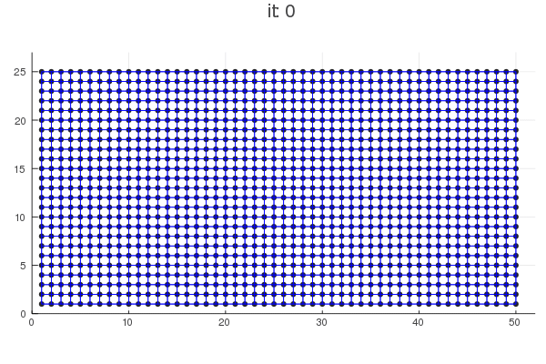
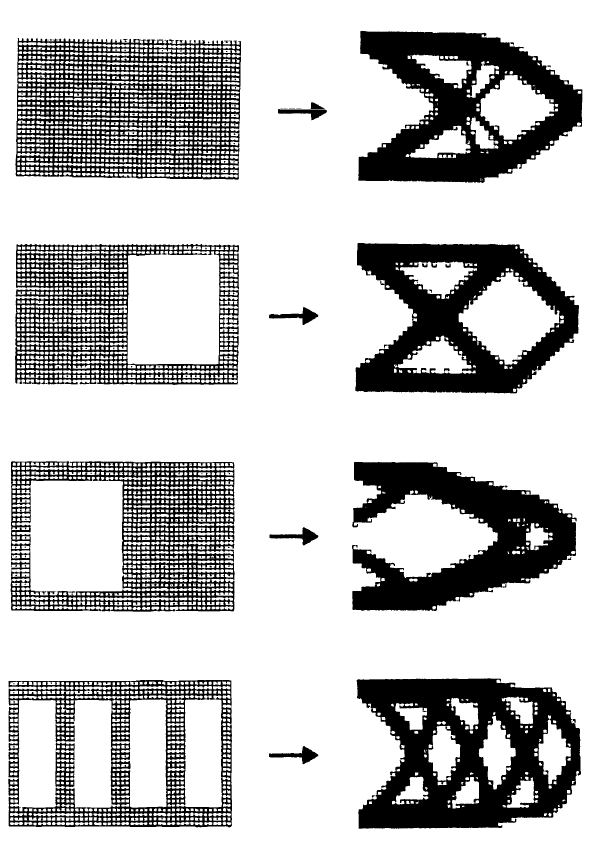
Local Opimization: Hybrid Cellular Automata
Approach:
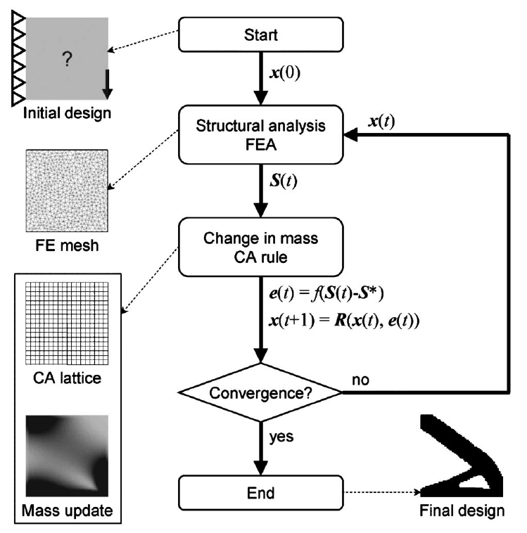
Algorithm:
- Define cells, load, fixed conditions
- calculate local stresses in cells
- change material properties of cells based on update rule:
Et+1=Et(1+α(σ/σc−1)
- Chang cell state ("death", "birth" or "division")
- return to step 2
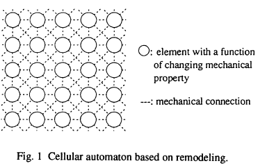
State αi of each cell is defined by design variables xi(t) (density,geometry,elastic modulus), and field variables Si(t) (stress, stain, strain energy density) (the relation between the amount of energy employed to deform a volume unit of a solid and imposed strain)).
αi={xi(t),Si(t)}
Strain Energy defined as follows:
U=i=1∑NUi,vi
Ui
Strain energy density, vi volume
The local minimization problem defined as:
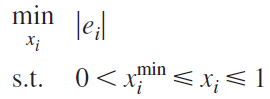
The error signal ei:
ei=Uˉi−Ui∗
Ui∗ is the local SED target,Uˉi is the average SED value:
Uˉi=N+1U1+∑j=1NUj
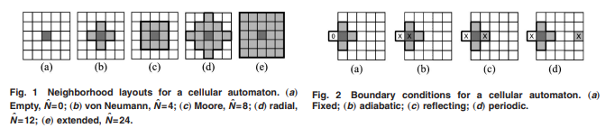
Neighborhood:
Local Control Rules:
- Two position control
Δxi(t)=cT∗sgn[ei(t)]
- Proportional control
Δxi(t)=cp∗ei(t)
- Derivative control
Δxi(t)=cd∗(ei(t)−ei(t−1))
- Integral control
Δxi(t)=cI∗τ=0∑t(ei(t−τ))
Algorithm:
- Define design domian, load cases, fixed conditions
- Define field variables (Simulation)
- calculate error signals
- Apply local rules and update the design variables
- check for convergence if not return to step 2
Implementation of HCA
Jupyter Notebook
Next Steps